

Introduction
Industrial load shifting often begins with a frustrating discovery: the electricity bill shows when the factory peaked, but not which production step caused it or whether that step could safely move. That missing link matters. If a supplier sizes a battery from the gross site peak before understanding compressors, chillers, tanks, cleaning cycles and production buffers, the factory may buy capacity that operations could have released at lower cost.
The variation between factories is too large for a generic rule. A 2017 study of four German manufacturing SMEs found technical load-shifting potential ranging from about 35 kWh to 848 kWh per day. The authors identified machine type, production strategy and scheduling flexibility as major reasons for the difference. That range is not an industry average; it is evidence that the work must start with the site, not a percentage copied from another project. The findings are reported in the peer-reviewed study “Load-shifting potential at SMEs manufacturing sites”.
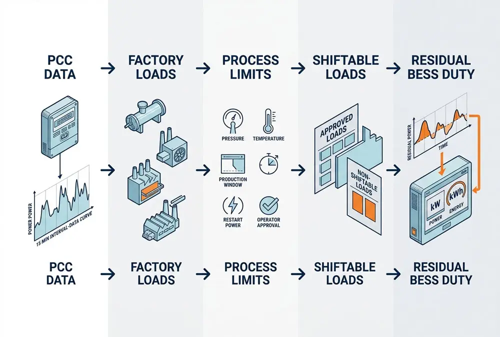
The practical answer: list each major load, its measured kW, energy per cycle, allowed operating window, process-state limits and recovery requirement. Shift what production can move safely. Use process buffers where they already exist. Only then calculate the residual power-versus-time duty that may require C&I energy storage.
This article gives you that inventory method, a worked factory calculation and a defensible route from load data to a preliminary BESS screen.
Map the Factory First
Start at the PCC
Start with the point of common coupling (PCC), the electrical boundary where the site’s grid import is measured. Collect at least 12 months of interval data, the applicable tariff or supply contract, and the transformer or contractual import limit. Monthly kWh totals are not enough. They cannot show whether a 700 kW peak lasted three minutes, one 15-minute billing interval or two hours.
Align the timestamps before drawing conclusions. A plant controller may sample every second, a sub-meter every minute and the bill at a longer settlement interval. If those records use different time zones, daylight-saving rules or clock synchronization, a convincing-looking load-shifting result can be assigned to the wrong production event. Aggregate the high-resolution data to the actual billing interval, but keep the original resolution for control and restart analysis.
This is where a common buyer problem appears: the site manager knows Tuesday at 14:15 was expensive, but cannot identify the responsible line. Installing meters everywhere is rarely the best first move. Use the PCC curve to isolate the largest recurring events, then sub-meter the compressors, chillers, ovens, pumps or lines most likely to create them. The IEA 4E EMSA report “Digitalisation in motor systems – Part I” (2024) describes industrial examples that use line-level electricity and compressed-air monitoring to turn factory data into operating targets.
Test the Data Before the Load
A load model can be mathematically correct and still use the wrong evidence. Before calculating flexibility, test coverage, time alignment and measurement boundaries. For 30 days of 15-minute data, the expected record count is 30 × 24 × 4 = 2,880 intervals. If 72 intervals are missing, coverage is:
Data coverage = (2,880 − 72) ÷ 2,880 = 97.5%
That percentage is not automatically acceptable. If the 72 missing intervals contain line startups or the monthly maximum, the dataset may still be unusable for sizing. Inspect where the gaps occur, not only how many exist.
- Coverage: valid intervals divided by expected intervals, with missing peak periods identified.
- Clock alignment: compare PCC, sub-meter and production timestamps during a known start or stop event.
- Boundary: confirm whether the reading is whole-site import, one feeder, one line or one machine.
- State context: join energy records to product, batch, shift and machine-state data rather than analysing an anonymous load curve.
A quotation based only on monthly bills is not a factory flexibility study. It may be enough for a discovery conversation, but not for a guaranteed kW reduction or BESS configuration. Ask the EPC to name the interval dataset, missing-data treatment, PCC boundary and production states used in its model.
Record Production States
Do not map only hours of the day. Map production states: normal output, startup, batch heating, cleaning, changeover, maintenance, weekend standby and recovery after an unplanned stop. A factory peak is often a production-state event rather than a clock event. Two compressors may coincide because a line restarted late; an oven may heat at the same time as chilled storage recovers from loading. A fixed 17:00–19:00 control schedule will miss events that move with the order book.
- Mark the product, batch or shift associated with each target event.
- Record what happened immediately before the peak, not just during it.
- Measure the recovery period after a load is delayed or curtailed.
- Ask production who can authorize a change and how quickly it can be reversed.
If you need a deeper explanation of grid-facing peaks before building this map, the guide to how peak shaving changes measured C&I demand explains the difference between kW, kWh and the billing interval.
Classify the Loads
A load is not flexible merely because it can be switched off. The useful question is whether its electrical demand can move while safety, product quality, throughput, labour and delivery commitments remain acceptable. This is a point where energy and production teams often talk past each other: the energy manager sees 120 kW available; the production manager sees a pressure drop, a line restart and a late order. If those consequences are absent from the model, production will rightly reject the control strategy. The German SynErgie white paper “Industrial Flexibility Options and their Applications in a Future Energy System” (2021) distinguishes organisational measures, such as adapting production planning, from technical measures that change a machine- or process-specific load profile. That distinction is useful on the factory floor.
| Load Class | Factory Example | Evidence Required | Risk if Misclassified | Buyer Benefit |
|---|---|---|---|---|
| Flexible | A non-urgent cleaning or pumping cycle with a wide completion window | Measured kW, run time, earliest start and latest finish | Several “flexible” jobs are moved into the same new peak | Direct scheduling may release capacity without battery cycling |
| Conditional | Compressed air, chilled storage or a heated process tank | Pressure, temperature, buffer level, restart and quality limits | The process crosses its safe boundary or rebounds aggressively | Existing process buffers can provide measured flexibility |
| Fixed or critical | Safety ventilation, an active continuous process or a quality-critical line | Process hazard review, continuity requirement and restart consequence | Scrap, downtime, unsafe conditions or missed delivery | Keeps operational risk out of the savings model |
Find the Storage Already in the Process
Some industrial processes already contain a usable buffer. Compressed-air pressure, a chilled room, a heated cleaning tank, thermal mass or intermediate material stock can temporarily decouple electricity use from production output. This does not make the process a battery, but it may let the electrical input move within a controlled range.
A 2020 study from Technical University of Darmstadt, “Quantifying the Demand Response Potential of Inherent Energy Storages in Production Systems”, modelled these process buffers and applied the method to a metalworking production line. The researchers used water temperature in an electrically heated cleaning tank and pressure in the compressed-air network as state indicators. For a factory buyer, the lesson is practical: add the process state to the load inventory. A kW reading alone cannot tell you how long the asset may safely wait.
Reported European examples—not universal benchmarks
- The IEA 4E EMSA report describes a Swedish cold-storage project where shifting refrigeration to nighttime reduced peak-period load by 50%; load shifting combined with other operational measures produced a reported 20% electricity reduction.
- The same report describes base-load management at BMW’s Steyr plant, reporting reductions of 52% of the original electrical base load and 14% of the compressed-air base load.
These are site-specific reported results. They show what measurement and operating discipline can uncover; they are not forecasts for another factory.
Build the Load Inventory
The inventory should be useful to production, finance and an EPC—not just to the person who exported the meter file. Keep one row for each material process or controllable asset. Record its owner, measured power, energy per cycle, allowed shift window, minimum on/off time, ramp or restart power, process state, recovery energy, production consequence and control interface. If several machines always operate as a single production cell, group them and document the control boundary.
The example below is an illustrative factory dataset. Its values were selected to demonstrate the method; they are not measurements from an AnengJi customer, a market average or a product guarantee.
| Factory Load | Measured Duty | Allowed Shift | Process / Rebound Evidence | Classification | Decision |
|---|---|---|---|---|---|
| Air-compressor bank | 120 kW × 60 min = 120 kWh | Up to 20 min | Pressure band 7.2–8.0 bar; 150 kW restart | Conditional | Test staged control; cap recovery power |
| Chiller plant | 90 kW × 120 min = 180 kWh | Up to 45 min | Product temperature 4–6°C; 105 kW recovery | Conditional | Validate thermal hold time by season and batch |
| Parts-cleaning cycle | 45 kW × 40 min = 30 kWh | 3-hour completion window | Tank temperature 60–70°C; no extra restart spike | Flexible / conditional | Schedule directly if temperature remains valid |
| Batch oven | 220 kW × 75 min = 275 kWh | 15 min before recipe risk | Recipe temperature and delivery slot are binding | Fixed for current plan | Do not dispatch without production requalification |
| Safety ventilation | 35 kW continuous | None | Safety function; no acceptable interruption | Critical | Exclude from savings and flexibility totals |
The three potentially movable duties above total 330 kWh per operating cycle, but 330 kWh is not automatically available during one target event. Their time windows, process states and recovery periods may not overlap. Put every candidate on the same timeline before summing it. Procurement teams often receive a large “flexible energy” total that disappears when production timing is applied.
Do not hide unknowns. If a machine has no sub-meter, label its load as estimated. If production has not approved the shift window, mark it unconfirmed. A smaller inventory with visible evidence gaps is more useful than a polished spreadsheet full of assumed flexibility.

Calculate the Shift Window
Separate Power From Energy
The first reproducible calculation is simple:
Shifted energy (kWh) = average shifted load (kW) × shift duration (h)
Illustrative example: moving a 150 kW compressor duty for 90 minutes shifts 150 kW × 1.5 h = 225 kWh.
That does not automatically save 225 kWh. Unless the task is eliminated or made more efficient, much of that energy will be consumed later. The economic result depends on the price or network signal, losses, recovery conditions and any production cost created by the move.
Check Rebound and Coincidence
A “valley” on the tariff is not necessarily spare electrical headroom. Night refrigeration, compressed-air recovery, EV charging or the next shift’s startup may already use the transformer capacity. Suppose the moved process restarts at 180 kW while 400 kW of other production load is running. The new coincident demand is:
180 kW + 400 kW = 580 kW
If the site import ceiling is 550 kW, the rescheduled process creates a new 30 kW breach. Cap the recovery power or move the task again; do not call the original shift a success.
This is also why peak shaving and load shifting need different success metrics. The C&I strategy comparison explains when the costly quantity is maximum kW and when it is time-specific kWh.
Use the FLEX-5 Screen
Before a load enters the dispatch plan, score five evidence areas from 0 to 2. This is an original planning screen, not an industry standard or product ranking.
- Freedom: Is there a documented time window, not just a verbal assumption?
- Load visibility: Is power measured at a useful interval?
- Effect on production: Are quality, throughput and labour consequences known?
- eXecution readiness: Can the action be controlled, logged and reversed safely?
- Five-data proof: Are power, energy, time window, process state and recovery documented?
A low score does not mean the load is permanently inflexible. It means the evidence is not ready for an investment decision. Add the missing meter, process limit or production approval before assigning value.
Size the Residual Duty
Once production-approved flexibility is known, subtract it from the target grid event. What remains is the residual duty. This is the point where C&I energy storage may enter the design—not before. Factory floor area, employee count and monthly consumption cannot define that duty on their own.
A Medium-Load Factory Example
Consider an illustrative factory that normally imports 450–520 kW at the PCC but repeatedly reaches 720 kW for 75 minutes when production lines, compressed air and cooling overlap. The site wants to hold grid import at 600 kW during that event. It therefore needs a gross reduction of 720 − 600 = 120 kW. “Medium-load” describes this example’s electrical profile only; it is not a universal classification by building size or industry.
Illustrative 75-minute factory event
Production can move part of the 120 kW target, but not for the entire event:
- Minutes 0–30: 80 kW of approved process load can move, leaving 40 kW for the BESS. Energy: 40 × 0.50 = 20 kWh.
- Minutes 30–45: only 50 kW remains shiftable, leaving 70 kW. Energy: 70 × 0.25 = 17.5 kWh.
- Minutes 45–75: production needs all shifted loads back, so the BESS carries the full 120 kW. Energy: 120 × 0.50 = 60 kWh.
Residual delivered energy at the PCC: 20 + 17.5 + 60 = 97.5 kWh.
Residual peak power: 120 kW. The average residual power is not the PCS requirement.
This gives the factory a useful first reference point: the relevant duty is not “a battery for a 720 kW factory.” It is a system capable of covering a 120 kW residual peak and delivering 97.5 kWh at the PCC across the defined event. A system close to 100 kWh may look sufficient on energy, yet fail because its inverter cannot deliver 120 kW—or because nominal DC capacity is being compared with delivered AC energy.
The example is deliberately simple. A real study must repeat the calculation across representative production days, abnormal starts, seasonal cooling loads and the available recharge window. The next-stage model must also account for usable state-of-charge limits, conversion losses, auxiliary consumption, temperature, degradation, reserve and warranty conditions. That is why two factories with the same 720 kW peak can need different storage systems.
Convert PCC Energy Carefully
For an initial screen, the nominal DC energy must be greater than the delivered AC energy because only part of the battery’s nominal capacity reaches the PCC. A simplified relationship is:
Initial nominal DC energy ≥ delivered AC energy ÷ (usable SOC fraction × discharge-path efficiency)
Illustrative base case: 97.5 kWh ÷ (0.90 × 0.90) = 120.4 kWh nominal DC.
This result still excludes protected backup reserve, end-of-life degradation allowance and abnormal auxiliary demand.
The same 97.5 kWh PCC duty produces materially different preliminary capacities when assumptions change:
High usable case
95% usable × 92% path efficiency
97.5 ÷ 0.874 = 111.6 kWh
Base screen
90% usable × 90% path efficiency
97.5 ÷ 0.810 = 120.4 kWh
Conservative screen
80% usable × 88% path efficiency
97.5 ÷ 0.704 = 138.5 kWh
These are engineering assumptions for sensitivity analysis, not published AnengJi product efficiencies. A supplier should replace them with guaranteed values at the agreed AC/DC boundary and performance date. If a quotation presents only nominal kWh and does not state the usable AC delivery obligation, return it for clarification.
Screen Products After the Duty
The product comparison now becomes meaningful. AnengJi’s published 100.48 kWh cabinet options list rated AC outputs of 30, 40 or 50 kW. One cabinet would therefore fail the illustrative 120 kW residual-power requirement. Its nominal energy is also below the 120.4 kWh base screen before adding reserve or degradation allowance. This is exactly why nominal kWh should not drive selection.
A published 210 kW / 418 kWh European C&I configuration clears the example’s first power-and-energy screen on paper. It is still not an automatic recommendation. The project must verify usable AC energy at the agreed boundary, the 800 V AC interface, reserve strategy, recharge window, auxiliaries, controls, protection, grid connection and proposal-specific warranty.
For a complete battery calculation after the factory inventory is approved, use the dedicated load-shifting energy-storage guide. Keep the load inventory as the operating input; do not replace it with a standard factory-size range.
Not Sure What Can Move?
Share your interval data, production schedule and major-load list. An initial review can identify missing inputs and define the residual duty that a BESS proposal should address.
Keep Market Value Local
The physical inventory travels well across Europe and the United States; the monetary value does not. Germany, other EU countries, the UK and individual US utilities can use different capacity charges, time-of-use periods, demand intervals, dynamic-price exposure and demand-response rules. A load may be technically shiftable but commercially worthless under the actual contract—or valuable for a different reason, such as avoiding a connection upgrade.
Keep three values separate: the energy moved, the peak demand reduced and any market service delivered. Do not add their gross values if they require the same load or battery capacity at the same time. For a European project, model the specific country, supplier/network tariff and metering boundary. For a US project, use the actual utility rate and programme rules rather than a national demand-charge assumption.
Calculate Gross Value Before Payback
The inventory becomes commercially useful when each physical action is mapped to the exact bill component. The following illustration uses assumed prices only to show the calculation; €0.12/kWh and €0.20/kWh are not European market averages or quotations.
Direct process shift
225 kWh × (€0.20 − €0.12) × 220 eligible days = €3,960 gross annual energy value, before labour, production, metering or control costs.
Battery-mediated shift at 90% assumed AC-to-AC efficiency
Required charge energy: 225 kWh ÷ 0.90 = 250 kWh.
Avoided high-price purchase: 225 × €0.20 = €45 per cycle.
Charging cost: 250 × €0.12 = €30 per cycle.
Gross spread value: (€45 − €30) × 220 = €3,300 per year, before degradation, auxiliaries, maintenance, financing, taxes and availability.
This comparison exposes a pain point that is often hidden in sales models: moving the process and using a battery are not economically identical, even when they shift the same delivered kWh. Direct scheduling may have lower electrical losses but a higher production cost. A BESS may protect the production timetable but introduces losses and asset costs. Model both routes against the same event before deciding.
Demand-based value needs a separate formula: verified kW reduction × the applicable capacity or demand rate × eligible billing periods. Do not add that value to energy-shift value until the dispatch simulation proves both outcomes can be delivered by the same asset without double-allocating power, energy or process flexibility.
Connect Production Signals
Move Beyond a Timer
A factory EMS needs more than a tariff calendar. Useful inputs can include PCC power, the applicable price or demand threshold, PV forecast, process temperature or pressure, MES job state, machine availability, BESS state of charge and the site import ceiling. The controller should know both what is cheap and what production is doing.
This is where many projects lose the confidence of operators. A schedule works during commissioning, then a late batch or line stoppage changes the load sequence. The EMS shifts the wrong process or empties the battery before the real peak. The solution is not simply a better forecast. Use production-state signals where available, log the reason for every action and define a local fallback that keeps the plant safe if a signal disappears.
Define Safe Fallbacks
- If PCC data is stale, stop automatic load increases and revert to the approved local limit.
- If the MES or SCADA state is unavailable, do not assume the process is flexible.
- If production rejects an action, preserve the reason code for later model improvement.
- If the battery or controllable load is unavailable, prevent other services from allocating the missing capacity.
- Begin with advisory or operator-approved actions where the production consequence is uncertain.
The EU-funded FLEX4FACT Guidebook on Flexibilization of Industry emphasizes formal production constraints, data feeds, baseline preparation, user acceptance testing and defined roles for planners, process teams and energy managers. Those implementation details are more important to reliable industrial load shifting than a sophisticated optimizer operating on incomplete data.
Prove the Result
A successful dispatch needs two records: the electrical result and the production result. Measure the same PCC boundary and billing interval before and after the action. Also log the commanded change, actual kW response, duration, recovery energy, process state, output and any quality or labour consequence.
This avoids a familiar argument at acceptance: the EMS dashboard reports energy shifted, finance sees no reduction in the costly bill line and production remembers the recovery overtime. All three can be correct if they are measuring different outcomes. FLEX4FACT’s verification approach uses real-time acquisition and event tracking so delivered flexibility can be audited. Apply that logic inside the factory before claiming savings.
The uncomfortable but useful rule is this: if the project cannot reproduce the event at the PCC and show what production did at the same time, it cannot prove the claimed benefit. A dashboard screenshot is not an acceptance test. Agree the baseline days, exclusion rules, timestamp source and production-normalisation method before commissioning—not after finance challenges the first savings report.
- Electrical acceptance: delivered kW, shifted kWh, PCC limit compliance and time-synchronised logs.
- Process acceptance: no unapproved quality, throughput, safety or restart consequence.
- Control acceptance: reason-coded commands, recoverable fallback and operator override.
- Commercial acceptance: the result is mapped to the actual tariff, contract or avoided infrastructure constraint.
Prepare the Site Data Pack
When the inventory is ready, an EPC or BESS supplier should receive more than a monthly bill. Send a consistent data pack:
- 12 months of interval import/export data and electricity bills;
- the tariff, demand interval and contractual power limit;
- the single-line diagram, transformer rating and known connection constraints;
- the production calendar and completed shiftable-load inventory;
- PV or other on-site generation data, with AC/DC ratings identified;
- critical-load and backup-reserve requirements;
- available PLC, MES, SCADA and EMS interfaces, including cybersecurity restrictions.
Ask the supplier to return the residual duty at the same PCC boundary, the proposed AC power, usable AC energy, recharge plan, reserve allocation and test method. That makes quotations comparable and prevents process flexibility from being counted once as avoided load and again as battery value.
Turn the Inventory Into a Design
AnengJi can review the measured residual power, duration, recharge window and site constraints, then discuss a suitable C&I storage configuration. Final capability depends on the selected equipment, electrical design and project verification.
Industrial Load Shifting FAQs
What is industrial load shifting?
It is the planned movement of controllable industrial electricity demand to another time while respecting production, safety, labour and quality constraints. It normally changes when energy is used rather than removing the task.
Which factory loads are easiest to shift?
Utilities and buffered processes—such as selected pumping, compressed air, refrigeration, cleaning or thermal duties—may offer flexibility. Suitability still depends on measured power, the process-state limit, minimum run time, restart behaviour and production approval.
Does load shifting reduce energy use?
Not necessarily. The main action changes timing. Total energy can remain similar, increase because of recovery or storage losses, or decrease when the new operating period improves process efficiency. Report shifted and avoided energy separately.
Is a battery required?
No. Production scheduling, direct load control and thermal or process buffers may shift part of the demand. A BESS is useful when the remaining event cannot move operationally, production must continue or storage provides another verified service.
Can load shifting create a new peak?
Yes. Delayed processes, compressed-air recovery and battery charging can coincide later. Model the recovery load, cap grid import at the PCC and test abnormal production days before automating the strategy.
How much data is needed?
Begin with 12 months of site interval data and the production calendar. Then meter the largest or most uncertain contributors to target events. The required resolution depends on the billing interval, equipment dynamics and control objective.
When should a factory consider BESS?
Consider BESS after the valuable residual power-versus-time event is measured, the tariff or connection benefit is verified, and the recharge window is feasible. Size power and usable energy separately; factory size or monthly consumption alone is not enough.
Related Articles
- Calculate load-shifting storage power, energy and recharge
- Understand peak shaving at the billing meter
- Choose between peak shaving and load shifting
- Review C&I battery system configurations
Sources and Evidence
- Pechmann et al. (2017), Load-shifting potential at SMEs manufacturing sites.
- IEA 4E Electric Motor Systems Platform (2024), Digitalisation in motor systems – Part I.
- SynErgie/Fraunhofer-affiliated research partners (2021), Industrial Flexibility Options and their Applications in a Future Energy System.
- Strobel et al., Technical University of Darmstadt (2020), Quantifying the Demand Response Potential of Inherent Energy Storages in Production Systems.
- FLEX4FACT, EU Horizon Europe, Guidebook on Flexibilization of Industry.

 https://anengjipower.com/wp-content/uploads/2026/06/epc-vs-turnkey-solar-project-bess.webp
675
1000
Charging Station Engineer
https://anengjipower.com/wp-content/uploads/2025/09/anengji-dc-fast-charging-station-manufacturer-and-supplier-logo-white-1.png
Charging Station Engineer2026-06-22 07:16:042026-06-24 07:13:17What Is the Difference Between EPC and Turnkey Contract Models in Energy Projects?
 https://anengjipower.com/wp-content/uploads/2026/06/anengji-commercial-solar-plus-storage-benefits-site.webp
675
1000
Charging Station Engineer
https://anengjipower.com/wp-content/uploads/2025/09/anengji-dc-fast-charging-station-manufacturer-and-supplier-logo-white-1.png
Charging Station Engineer2026-06-20 14:34:102026-06-20 14:37:43What Are the Top Benefits of Solar Battery Storage in Factories?
 https://anengjipower.com/wp-content/uploads/2026/06/modular-commercial-solar-battery-storage-cabinet.webp
675
1000
Charging Station Engineer
https://anengjipower.com/wp-content/uploads/2025/09/anengji-dc-fast-charging-station-manufacturer-and-supplier-logo-white-1.png
Charging Station Engineer2026-06-18 09:16:522026-07-03 03:05:13What Is Solar Battery Storage? Complete C&I Engineering Guide


Leave a Reply
Want to join the discussion?Feel free to contribute!